Analysing Pelton distributors

During construction of the Kopswerk II pumped storage power plant in Austria, the design for the Pelton distributor was developed on the basis of computational fluid dynamics (CFD) and finite element analyses (FEA).

Only a few years ago, the verification of the analytical stress calculation as described in [1], [2], [3], [4] and [5] for a distributor as a standard component was executed using a shell model (also described in [5], [6] and [7]) which included the first bifurcation, as the largest and normally most critical one. New possibilities in analysis techniques in CFD and FEA allow for optimised solutions which deviate from the standard. They ask for a careful verification of stress and displacement, and as a result of increased hardware and software potential, more sophisticated analyses are possible, as is shown in the following paper.

Using as an example the Pelton distributor at Kopswerk II, the paper shows how the calculation models have changed from shell models of the first bifurcation to solid 3D-models of the whole distributor. Finally, an analysis of the solid 3D-model under consideration of the surrounding concrete will be investigated to discover if possible additional stresses due to the adapted boundary conditions would need to be considered in the design of a distributor.

Material model

Throughout the analyses a linear elastic material behaviour was applied for steel and concrete. This is justified since in the case of the distributor the calculated stresses are sufficiently below the plasticity range. Regarding the concrete, the boundary conditions have been chosen such that nearly no tension will be transferred to the surrounding concrete.

Finite element models and boundary conditions

The shell model

The basis for the shell model (Figure 1) is a 3D-area model of the first bifurcation. It has been built up with the shell element SHELL93 which is particularly well suited to modelling curved shells. The element has six degrees of freedom at each node: three translations and rotations. The approach of the deformation shapes is quadratic in both in-plane directions. The shell elements in Figure 1 are displayed as solids with the shape determined from the real constants (thickness).

The boundary conditions are defined as displayed in Figure 1: fixed support at the inlet of the bifurcation and symmetric behaviour on the cut boundaries. The internal pressure corresponds to the design pressure which is the sum of the static pressure including water hammer. The distributor is designed as a covered self-supporting containment, i.e. all forces can be endured by the structure itself, which is in correspondence with the dimensioning philosophy.

The solid model

The solid model (Figure 2) is based on a 3D-CAD volume of the whole distributor and consists of SOLID187 tetrahedral elements, defined by a quadratic displacement approach and well suited to modelling irregular meshes. The element is defined by 10 nodes, having three degrees of freedom each, with the translations in the nodal x, y, and z directions.

The boundary conditions are the same as in the case of the shell model and are displayed in Figure 2.

The solid model with concrete

The solid model with concrete (Figure 3) consists of SOLID187 tetrahedral elements – the same as the solid model. In addition, the contact between distributor and concrete is modelled with the contact element CONTA174 and the target element TARGE170. The CONTA174 is used to represent contact between the 3D target surfaces (TARGE170) and a deformable surface, defined by this element. This element is located on the surfaces of 3D solid or shell elements with midside nodes. TARGE170 is used to represent various 3D target surfaces for the associated contact elements (CONTA174). The contact elements themselves overlay the solid elements describing the boundary of a deformable body and are potentially in contact with the target surface, defined by TARGE170. For flexible targets, these elements will overlay the solid elements describing the boundary of the deformable target body.

The boundary conditions are shown in Figure 3. The contact between distributor and concrete is modelled with non-linear contact behaviour. The friction coefficient is taken from [8] and is 0.3. The gap between the contact surfaces is applied such that nearly no radial forces due to the internal pressure are transferred to the concrete. It reflects that the containment is self-supporting and the concrete should be loaded by longitudinal forces only. This results in a maximum stress regarding the Von Mises equivalent stress at the distributor.

As a consequence of the sophisticated task (non-linear contact analysis) only the first two bifurcations are taken into account. This is adequate since only the first bifurcation will be subject of the investigation.

Comparison and discussion of the calculation models

There are some circumstances one must consider when modelling with shell elements: The shell model is very useful when the structure is thin-walled and when applying standards or codes based on stress categories (primary and secondary stresses) like ÖNORM or ASME Code, because the several stresses can be postprocessed directly. But some difficulties regarding modelling appear when the wall thicknesses increase (also mentioned in [7]) which can be seen in Figure 4. One difficulty appears at the sickle (Figure 4a). Due to the fact that only the midplanes of the shell model are connected at these locations it is clear that there are some discontinuities regarding the local stiffness. A similar problem arises at locations where pipes of different wall thicknesses are connected (Figure 4b). In real structures there has to be a smooth transition on the inner surface due to the flow. Hence, there is a chamfered transition on the outer surface. With shell elements it is a demanding task to model a gradual increase of wall thickness including a smooth transition of the connected midplanes. This clearly results in a huge modelling effort and allows only a limited level of automation.

When modelling with general shell elements (SHELL93) there is always a stepped transition of the inner and outer surface whereas in real structures there is a chamfer or a smooth transition. Additionally, only the midplanes are connected. Nevertheless, these approximations in geometry and stiffness are justified when dealing with models having thin walls.

However, the mentioned approximations become significant with increasing wall thickness, as is the case at Kopswerk II. However, these problems can be avoided by using a solid model which takes all problems with stiffness and geometry into account. Generally, solid models are a closer approach to reality than shell models, but they are less convenient when handling stress categories.

After analysing the solid model, it is obvious that the next step is the inclusion of the surrounding concrete to get more insight into ‘reality’. It is important to know what additional stresses may arise due to the new boundary conditions.

Results of the finite element analysis

Total displacements

The results of the analysis at the first bifurcation are displayed in Figures 5a-c. These figures show the total displacements under design pressure for the three different calculation models. The total displacement is the absolute value (length) of the displacement vector. As expected, the highest values have been found at the solid model with concrete. Due to the free boundary conditions at the distributor flange the total displacement is mainly a function of the gaps between distributor and concrete. The displacements for the shell and the solid model (without concrete) are rather similar. It is clear that there must not be a large difference because both models have nearly the same boundary conditions. However, as a result of the different behaviour of the elements (shell – solid) there are a few distinctions. The regions close to the sickle and at the sickle itself are particularly affected by the change in stiffness mentioned earlier.

Von Mises equivalent stresses

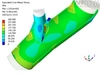
The results of the analysis at the first bifurcation are displayed on Figures 6a-c. These figures show the Von Mises equivalent stress under design pressure for the three different calculation models.

The differences of the stresses between the shell model and the solid model are a result of the geometric approximations as mentioned earlier. Figure 7 shows the membrane and the surface stresses at the symmetry plane at the inner edge of the first bifurcation. The membrane stresses are those stresses arising on the surface that bisects the thickness of the distributor wall. The surface stresses can be found on the outer and inner surface. Regarding the stress categories the membrane stresses and the stresses on the undisturbed surface are primary stresses. The surface stresses at the intersection lines where the pipes are connected are secondary stresses.

The reason why the paths displayed in Figure 7 have different lengths is because of the geometric differences between shell and solid model, especially at the regions near the intersection lines.

The diagram shows clearly that the difference between the shell and the solid model is negligible when the increase of wall thicknesses is small. Only at regions with a large increase of the wall thickness the differences become significant.

Figure 8 highlights the comparison of the stress results gained from the analysis of the solid models with and without concrete. The location of the path plot accords to the path plot in Figure 7.

The comparison of the path plots in Figure 8 shows an increase of the membrane and surface stresses at the undisturbed regions, i.e. between the intersection lines the stresses at the model with concrete are higher than without. This is clearly a result of the boundary conditions. As described earlier, the gaps between concrete and distributor were chosen such that the longitudinal forces are carried by the concrete. Thus the distributor is mainly loaded with hoop stresses; the longitudinal stresses are nearly zero. This results in a higher Von Mises equivalent stress.

At the intersection lines both the membrane and the surface stresses are nearly on the same level. The membrane stresses are slightly higher at the solid model without concrete whereas the surface stresses are slightly higher at the solid model with concrete.

The circumstance that the highest stresses are only slightly different indicates that the dimensioning philosophy of the covered self-supporting distributor design is a sufficiently safe design regarding the peak stresses which are relevant for life time calculations based on fatigue.

The authors are: Stefan Lais and Richard Angehrn, VA Tech Hydro, Hardstrasse 319, CH-8005 Zurich, email: Stefan.lais@vatech-hydro.ch; richard.angehrn@vatech-hydro.ch; and Josef Sugg, VA Tech Escher Wyss, Escher Wyss Strasse 25, D-88212, Ravensburg, email: Josef.sugg@vatew.de.